Annex 17. Applying summary measures of health inequality to individual data

Calculating the relative ranks of individuals

The calculations of the slope index of inequality (SII), relative index of inequality (RII), absolute concentration index (ACI) and relative concentration index (RCI) require individuals to be ranked from the least to the most advantaged, based on a socioeconomic characteristic such as wealth or education level. When the ranking is based on a continuous variable (e.g. wealth index scores), in which each individual has a unique score value, the formula to calculate relative rank is:

\[\text{Relative rank} = \sum_{i=1}^j p_i - 0.5(p_j)\]

where \(p_j\) is the individual sampling weight. An example is shown in Table A17.1.

TABLE A17.1. Steps to calculate the relative rank of individuals in a hypothetical weighted sample using a continuous ranking variable (wealth index score)

Record	Wealth index score	Individual sample weight [A]	Population share [C = A / B]	Cumulative population share [D]	Relative rank [X = D − (0.5 × C)]
						1	−250 248	1250	0.040	0.040	0.020
2	−111 979	2468	0.079	0.118	0.079
3	−34 038	1787	0.057	0.175	0.147
4	−29 844	8873	0.283	0.458	0.317
5	−7243	2202	0.070	0.528	0.493
6	8136	1084	0.035	0.563	0.546
7	32 187	7212	0.230	0.793	0.678
8	59 185	1875	0.060	0.853	0.823
9	88 405	3387	0.108	0.961	0.907
10	308 001	1238	0.039	1.000	0.980
Total		31 376 [B]

When the ranking variable is categorical (e.g. wealth quintiles or education level), resulting in ties in the ranking variable, the relative rank can be calculated from the proportion of individuals within a given value of the ranking variable. This produces a single relative rank per subgroup, rather than individually (due to not being able to accurately sort individuals within each subgroup). An example of this calculation is shown in Table A17.2.

TABLE A17.2. Steps to calculate the relative rank of individuals in a hypothetical weighted sample using a categorical ranking variable (education level)

Record	Education level	Individual sample weight [A]	Cumulative individual sample weight [C]	Cumulative individual sample weight for Record 1 [D]	Maximum cumulative individual sample weight per category [E = max(C)]	Minimum cumulative individual sample weight for Record 1 [F = min(D)]	Relative rank [G = (F + 0.5 × (E − F)) / B]
								1	No education	1250	1250	0	3718	0	0.059
2	No education	2468	3718	1250	3718	0	0.059
3	Less than primary education	1787	5505	3718	14 378	3718	0.288
4	Less than primary education	8873	14 378	5505	14 378	3718	0.288
5	Primary education	2202	16 580	14 378	17 664	14 378	0.511
6	Primary education	1084	17 664	16 580	17 664	14 378	0.511
7	Secondary education	7212	24 876	17 664	26 751	17 664	0.708
8	Secondary education	1875	26 751	24 876	26 751	17 664	0.708
9	Higher education	3387	30 138	26 751	31 376	26 751	0.926
10	Higher education	1238	31 376	30 138	31 376	26 751	0.926
Total		31 376 [B]

Calculating summary measures of health inequality

The following example measures inequality in child undernutrition among children in Kenya using data from the 2022 Demographic and Health Survey (DHS). The sample includes children aged five years and younger. Undernutrition is measured using negative height-for-age z-scores (which is related to stunting), censored at 0 and multiplied by −1. A larger absolute value of this measure indicates that a child’s height is further below the median height of a child of the same age and sex in a well-nourished population. Socioeconomic status is measured using the DHS wealth index, which is constructed from data about household assets and housing conditions.

Slope index of inequality and relative index of inequality

To calculate the SII and RII, undernutrition (height-for-age z-scores) is regressed against the fractional wealth index rank of each child in the survey. After running a regression model, the predicted child height-to-age estimates at the socioeconomic ranks of 1 and 0 are 0.63 and 1.47, respectively. The SII is the difference between these predicted estimates (or the slope of this line):

\[SII = \hat{v}_1 - \hat{v}_0 = 0.63 - 1.47 = -0.84\]

Since undernutrition is an adverse indicator, the negative sign indicates inequality favouring advantaged people – that is, the censored standardized height deficit of the poorest child is predicted to be 0.84 lower than that of the richest child.

The RII is the ratio between the predicted child undernutrition estimates at the socioeconomic ranks of 1 and 0:

\[RII = \hat{v}_1 / \hat{v}_0 = 0.63 / 1.47 = 0.43\]

Therefore, the poorest child has a height-to-age score that is 0.43 times lower than that of the richest child.

Absolute concentration index and relative concentration index

Figure A17.1 shows a concentration curve for child undernutrition in Kenya in 2022. It plots the cumulative proportion of undernutrition against the cumulative proportion of children ranked from poorest to richest. The curve lies above the 45-degree line, confirming that undernutrition is disproportionately concentrated among poorer children. The absolute concentration index is twice the area between the concentration curve and the 45-degree line.

FIGURE A17.1. Concentration curve: child undernutrition, Kenya

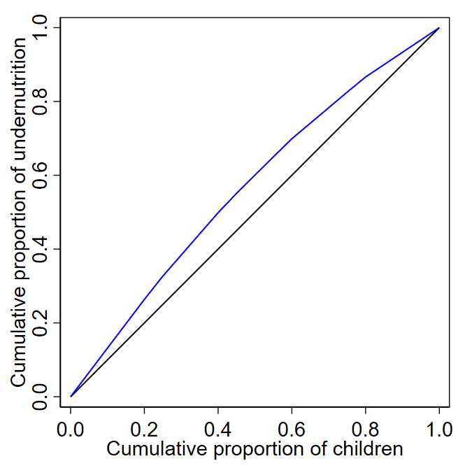
The black 45-degree line represents a situation of equality. The blue line represents the Lorenz curve, a situation of inequality.

Source: data were sourced from the 2022 Kenya Demographic and Health Survey.

The ACI is −0.1397 and the RCI is −0.1327. The negative sign indicates inequality in undernutrition, to the disadvantage of poorer children.