Chapter 25. Further quantitative inequality analysis approaches and measures
Overview
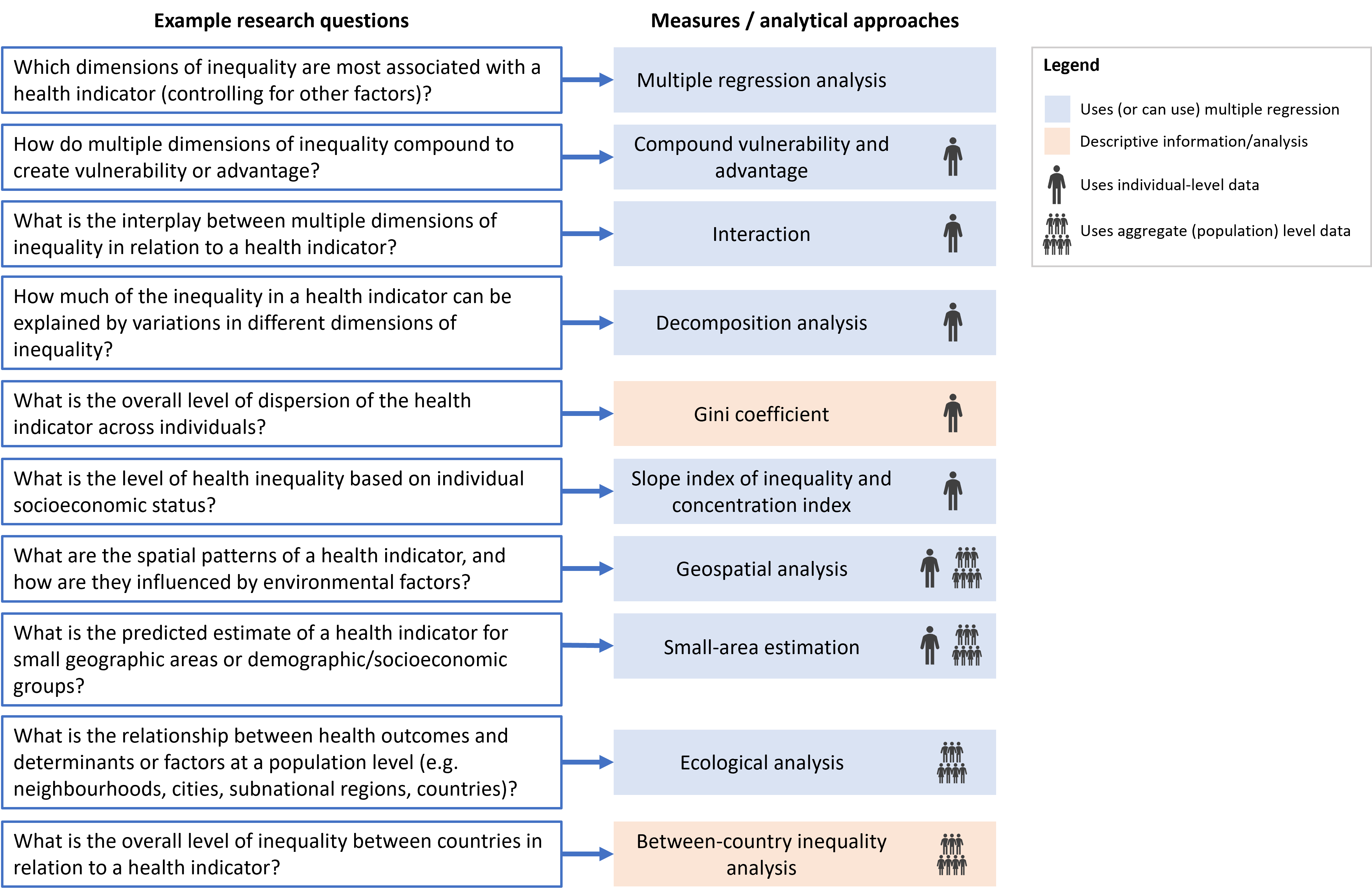
Health inequalities are driven by a complex system of demographic, socioeconomic, environmental and geographical factors. The approaches for analysing disaggregated data and summary measures of health inequality (see Chapters 17–23) quantify a bivariate relationship between a health variable and a dimension of inequality and can be used to gain initial insights into the patterns and magnitude of health inequalities related to one or more dimensions of inequality at a time. There are, however, other research questions about health inequalities that these methods cannot be used to answer. For example, which dimensions of inequality are most associated with a health indicator (controlling for the others)? What is the interplay between multiple dimensions of inequality in relation to a health indicator? How do environmental and spatial factors influence health inequalities? To answer these questions, other quantitative inequality analysis approaches and methods can be used.
This chapter explores examples of other health inequality monitoring research questions and demonstrates the application of common analytical approaches to answering them. After highlighting some initial considerations, the chapter introduces multiple regression analysis, which underpins many of the approaches discussed later. To answer research questions related to the dispersion of health indicators in a population or inequalities at the individual level, the chapter discusses measurement of inequality with individual-level data. The use of geospatial analysis and small-area estimation to answer research questions related to spatial and environmental inequalities is explored. Finally, the chapter addresses methods of exploring population-level inequalities, including ecological analysis of the associations between a health indicator and a health determinant, and the measurement of between-country inequalities. The approaches discussed in this chapter are not intended to be an exhaustive discussion of inequality analysis methods or a comprehensive resource for each. Detailed descriptions of these methods are available elsewhere (1–3).
Initial considerations
This chapter describes methods and measures used to answer some of the research questions that may arise from the analysis of inequalities using disaggregated data and summary measures of health inequality (Figure 25.1). When considering relationships between health indicators and health determinants, it is important to distinguish between association and causation. Many approaches discussed in this chapter assess associations (i.e. whether a health indicator is more likely in people with particular demographic, socioeconomic or geographic characteristics), and further analysis and investigation would be needed to establish causal links. The target audience and application of more advanced inequality analysis should always be considered. Analysts, researchers and others with expertise may need to be involved in interpretation of the findings to make them relevant to more general audiences.
FIGURE 25.1. Selected research questions and corresponding measures and analytical approaches
Multiple regression analysis
Regression analysis is used to gain a deeper understanding of intersectionality. Intersectionality is a concept describing the overlap of interconnected social identities (especially race/ethnicity, income/wealth and gender) and how this results in systemic discrimination or disadvantage (4). Studying intersectionality involves researching how dimensions of inequality overlap and intersect, resulting in differing experiences of health. Regression analysis can be used to research how multiple dimensions of inequality might compound to exacerbate vulnerability or advantage, estimate how they might interact to affect the health indicator, and estimate how much health inequality is driven by variations in different dimensions of inequality.
For more in-depth analysis, multiple regression analysis, or the analysis of multiple independent variables simultaneously, can be used to estimate the independent average effect of a characteristic (or dimension of inequality) on a health indicator, while accounting for all other observed dimensions of inequality. Multiple regression can support understanding of the dimensions of inequality that are most associated with a health indicator. Multiple regression analysis is used in several of the approaches discussed in this chapter. The multiple regression approach comes with several limitations – and even when a strong association is present, this does not necessarily indicate a causal link (3).
Multiple regression is a statistical technique used to analyse the relationship between a single dependent variable and several independent variables.
The choice of a particular regression model depends on the nature of the dependent variable (i.e. the health indicator). Linear regression is used when a dependent variable is continuous (e.g. height or weight). If the dependent variable is binary (i.e. measured as two possibilities – either not achieved or achieved, such as vaccinated versus non-vaccinated) or the relationship between the dependent and independent variables is nonlinear, logistic regression can be used. If the dependent variable is measured as a count (e.g. number of hospital admissions), Poisson regression or negative binomial regression can be used. There are also other forms of regression models (2, 3).
To run a multiple regression model, data about the health indicator and dimensions of inequality are needed for each unit of analysis (individual-level or population-level), and specialized statistical software is usually required. Practical and theoretical considerations also play an important role when formulating a regression model. First, developing a framework of variables to include in the regression model (e.g. using directed acyclic graphs (DAGs) (5)) requires some knowledge of the factors that could arguably be considered associated with health indicator. This is often guided by a literature review and the availability of data. Some other considerations are summarized in Box 25.1.
BOX 25.1. Considerations for formulating multiple regression models
The more independent variables that are added, the more the statistical power of the model decreases, due to smaller sample sizes for each possible combination of independent variables. A general rule is to limit the number of independent variables to less than the sample size divided by 10 (6). For example, to have six independent variables in the model, the sample size should be at least 60.
Multicollinearity is the condition in which there is a very high correlation between two or more independent variables in the model, resulting in unstable estimates because it is difficult to disentangle their individual effects on the dependent variable (7, 8). It is important to be aware of cases in which the same variable is (often inadvertently) used as both a dependent and an independent variable in the regression model (e.g. using a composite measure as an independent variable, which contains a component that is the same as or similar to the dependent variable).
If the data being analysed come from a survey, it is important to take survey design characteristics (e.g. individual sample weights, primary sampling units and strata) into account in the analysis (see Annex 8).
A multilevel model (also known as a hierarchical model or mixed-effects model) is a type of regression model that accounts for the clustering of individuals in a hierarchical or nested structure. For example, with household surveys, such as the Demographic and Health Surveys (DHS) or Multiple Indicator Cluster Survey (MICS) (see Chapter 12), individuals (level 1) are typically nested within districts (level 2), which are nested within states (level 3). One strength of a multilevel regression is its ability to quantify the proportion of the total residual variation (i.e. the unexplained variation in the regression outcome after accounting for covariate effects) lying at the various levels of the model’s hierarchy. For example, if a multilevel model includes individuals nested within districts, this allows the quantification of how much variation in a health indicator is related to individual-level factors (e.g. age, economic status or sex) versus district-level factors (e.g. air pollution rates, population density or public health-care funding).
The results of a regression analysis can be reported using different measures of association, such as absolute differences, odds ratios and prevalence ratios, where the outcome in one subgroup is compared against a reference subgroup within a given dimension of inequality. For example, the results from logistic regression analysis can be reported as odds ratios, where an odds ratio greater than 1 indicates that the characteristic is associated with higher odds of the outcome compared with the reference subgroup. For a health indicator where the goal is to achieve a maximum level (e.g. complete coverage of antenatal care), the reference subgroup selected could be the most disadvantaged subgroup (e.g. the poorest subgroup) so that odds ratios are generally greater than 1 and hence easier to interpret. When interpreting results, it is important to consider the uncertainty about the estimates using 95% confidence intervals and statistical confidence with the P value. Small sample sizes within subgroups, however, can increase the width of confidence intervals and affect whether results are statistically significant or not.
The WHO Explorations of inequality: childhood immunization report used logistic regression to analyse adjusted associations between immunization coverage with a third dose of diphtheria, tetanus toxoid and pertussis vaccine (DTP3) and selected demographic, socioeconomic and geographic characteristics in 10 countries (9). For example, Figure 25.2 shows the results from a household survey in Nigeria in 2013. Controlling for the other characteristics, a child aged one year in the richest quintile had a 7.3 times odds of being covered than a child in the poorest quintile; and a child whose mother had received more than secondary school education had a 6.6 times odds of being covered than a child whose mother who had received no education. The child’s sex, birth order and urban–rural place of residence showed nonsignificant association with DTP3 immunization coverage after adjusting for other factors (based on P≥0.05).
FIGURE 25.2. Adjusted odds ratios: immunization coverage with a third dose of diphtheria, tetanus toxoid and pertussis vaccine among children aged one year and background characteristics in Nigeria
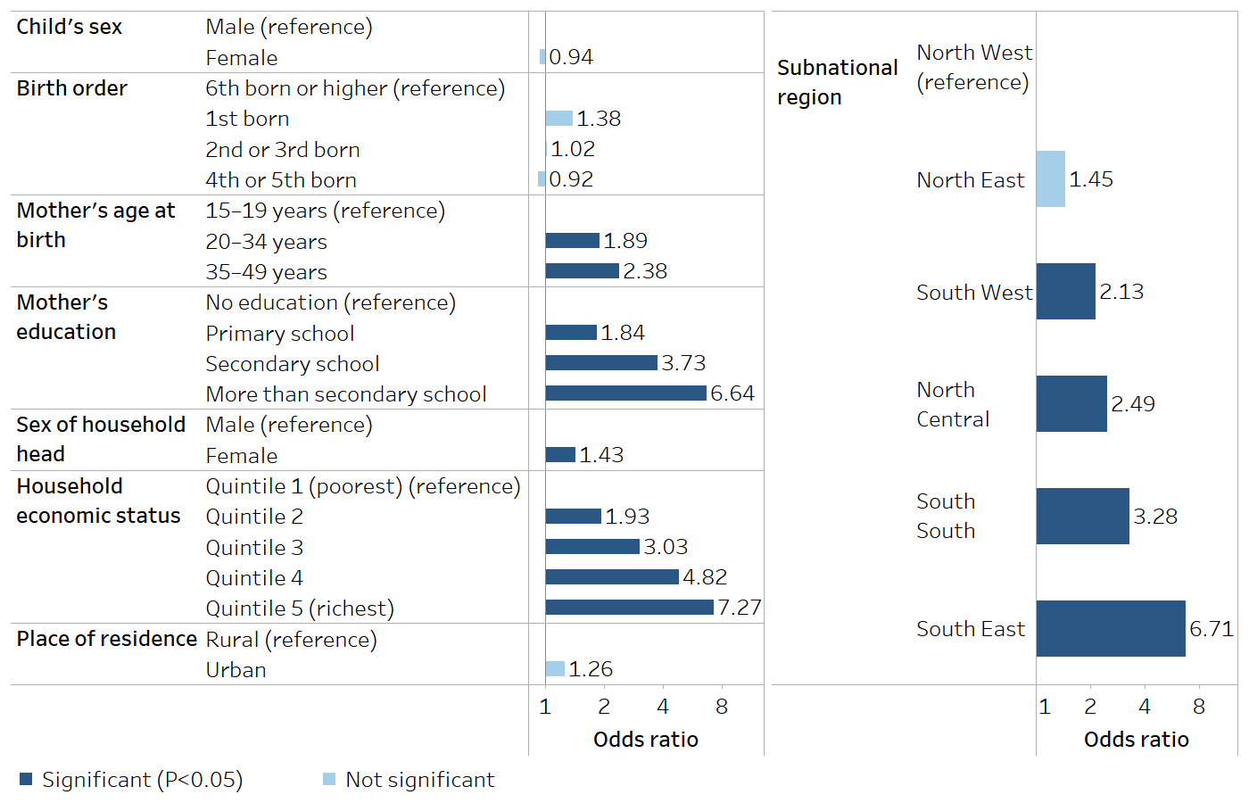
Source: derived from the WHO Explorations of inequality: childhood immunization report (9), with data sourced from the 2013 Demographic and Health Surveys.
Although multivariable regression methods are often used in inequality analysis to analyse associations between a health indicator and dimensions of inequality (rather than to establish causal links), controlling for confounding in regression models is important to obtain unbiased estimates. A confounding variable is a third variable that is related to the independent and dependent variables and that distorts the causal relationship between them. For example, when assessing the relationship between mortality rates among children aged under five years at the individual level and household economic status, the educational attainment of the child’s mother is likely a confounder of the relationship between economic status and under-five mortality because women with more education tend to live in wealthier households and their children experience lower mortality rates on average. Therefore, an analysis that ignores maternal education would likely lead to overestimating the protective effect of higher economic status by misattributing some of the protective effect of education to economic status. A confounding variable typically has a causal association with the dependent variable (e.g. if the dependent variable is a disease, it must be a risk factor or a protective factor for the disease); it must be distributed unevenly between the subgroups of the independent variable(s) (e.g. if age is a confounding factor for cancer mortality, it should be distributed unevenly among economic status subgroups); and it must not be part of the causal pathway between the independent variable(s) and the dependent variable (3). Literature reviews and DAGs are often used to guide the selection of confounding variables and enable them to be controlled for in the multiple regression analysis.
Compound vulnerability and advantage
Certain demographic, socioeconomic and geographic conditions can compound to exacerbate vulnerability or advantage. For example, how much more likely is a person to be unhealthy if they have a low level of education and have a low income and live in a rural area, compared with a person with higher education from a high-income household in an urban area? Summary measures of health inequality (see Chapters 19–22) cannot capture such differences arising from the effects of intersecting characteristics.
Compounding vulnerability or advantage could be assessed by stratifying the population into separate subgroups, each containing a combination of certain characteristics. A disadvantage of this approach is that subgroup sample sizes can get very small, affecting the robustness of the results. A simple approach to quantify compound vulnerability and advantage (when no interaction is present – see below) is to multiply the odds ratios of two or more associated factors from a logistic regression analysis.
Building on the previous example from the report Explorations of inequality: childhood immunization (Figure 25.2), in Nigeria in 2013, children with highly educated mothers aged 35–49 years who belonged to the richest 20% of the population had a 115 times odds of being vaccinated, compared with children born to teenaged mothers with no education in the poorest 20% of the population (9). The calculation method for this example is shown in Table 25.1. Interactions between the inequality dimensions were tested during the analysis (e.g. interactions between mother’s education and wealth quintile) and were not statistically significant (based on P≥0.05).
TABLE 25.1. Calculation of compound advantage using odds ratios from multiple regression analysis: immunization coverage with a third dose of diphtheria, tetanus toxoid and pertussis vaccine, Nigeria
|
Odds for more than secondary school education subgroup compared with no education subgroup [A] |
Odds for age 35–49 years subgroup compared with age 15–19 subgroup [B] |
Odds for richest quintile compared with poorest quintile [C] |
Compound advantage [A x B x C] |
|---|---|---|---|
| 6.64 | 2.38 | 7.27 | 114.89 |
Source: derived from the WHO Explorations of inequality: childhood immunization report (9), with data sourced from the 2013 Demographic and Health Surveys.
Interaction
One way to research the interplay between multiple dimensions of inequality in relation to a health indicator is through investigating interaction within a regression model. In regression analysis, interaction (or effect modification) means that the relationship between two variables changes, or is modified, depending on the value or a category of another variable. For example, when studying the relationship between smoking and income in a particular setting, it could be found that higher smoking prevalence is associated with lower income. Other factors, however, might change this relationship (e.g. sex). When an interaction is present, it would be incomplete to compute only an overall association without allowing for the fact that the association is different for people with or without the additional factor.
Multiple regression can be used to assess how the combined effect of income and sex on smoking prevalence differs from the sum of their individual effects that would be estimated from a model that did not allow for the interaction. Examining interactions between two independent variables in a regression model can be achieved via the inclusion of an interaction term (also referred to as a product term) that is the product of the two variables. The results of including an interaction term of income and sex would be similar to estimating the association between income and smoking within each sex.
Table 25.2 illustrates the example with empirical data from the World Health Survey conducted by WHO in 2003 (10). Data correspond to estimates from Ecuador and show the prevalence of smoking by sex and wealth quintile. The association between income and smoking is depicted by the relative index of inequality (RII) (which is calculated using a regression model, see Chapter 21), for which a value higher than 1 indicates inequality favouring the richest and a value less than 1 indicates inequality favouring the poorest. In this example, RII estimates differ substantially by sex, showing opposite associations between smoking and economic status. Among males there is a higher smoking prevalence at lower economic status, but the relation is inverse among females, with higher prevalence among the wealthier. Therefore, sex is considered an effect modifier.
TABLE 25.2. Relative index of inequality: smoking prevalence, by economic status, females and males, Ecuador
| Prevalence (%) | Relative index of inequality | ||||||
|---|---|---|---|---|---|---|---|
| Overall | Quintile 1 (poorest) | Quintile 2 | Quintile 3 | Quintile 4 | Quintile 5 (richest) | ||
| Males | 28.7 | 37.1 | 28.7 | 27.2 | 23.6 | 26.3 | 1.62 |
| Females | 7.1 | 4.2 | 5.5 | 5.8 | 8.3 | 11.8 | 0.28 |
Source: derived from Hosseinpoor et al. (10), with data sourced from the 2003 World Health Survey.
Decomposition methods
Decomposition methods can be used to answer research questions such as how much of the inequality in a health indicator can be explained by variations in different dimensions of inequality. These methods are usually based on linear regression models for two subgroups and by at least one dimension of inequality (e.g. regression of a health indicator by economic status, for urban and rural subgroups). Rather than producing the average estimate for each subgroup while controlling for the others (which is the output from multiple regression – see above), the output from decomposition methods quantifies the magnitude of the health inequality related to differences between specific population subgroups – for example, the difference in the health indicator between urban and rural residents.
Oaxaca–Blinder (O–B) decomposition is a method used to explain the gap in the means of a health indicator between two groups (e.g. between urban and rural, rich and poor, or female and male). It decomposes the observed health inequality into two components – group differences in the determinants included in the model (referred to as the explained component or endowment effects), and group differences in the partial associations of these determinants with the outcome (referred to as the unexplained component or discrimination effects) (1). It is crucial to note that the second component encompasses any associated differences arising from unobserved factors that are associated with both the outcome and the group indicator. The O–B decomposition method helps identify whether inequality in health between two groups arises from differences in the observable characteristics of those groups or from correlated unobserved factors (11).
For example, the O–B decomposition method can be used to estimate how much of the inequality in body mass index (BMI) between urban and rural residents of the Islamic Republic of Iran in 2011 was related to urban and rural differences in age, gender, physical activity and socioeconomic status (i.e. group differences, or the first component), and how much is driven by other factors (i.e. the second, unexplained, component). Two linear regressions – one for urban and one for rural residents – were estimated with BMI as the dependent variable and age, gender, physical activity and socioeconomic status as the independent variables. In Table 25.3, the difference in BMI between urban and rural subgroups was 1.16 points (BMI was 26.40 among urban adults and 25.24 among rural adults); 75% of this difference (0.87 of 1.16) was due to urban–rural differences in age, gender, physical activity and socioeconomic status, and the remainder of the urban–rural inequality was unexplained by the factors in the model. Differences in socioeconomic status between the urban and rural subgroups accounted for 72% (0.83 of 1.16) of the urban–rural inequality in BMI (11).
TABLE 25.3. Oaxaca–Blinder decomposition of place of residence inequality: body mass index (BMI) by place of residence, Islamic Republic of Iran
| Coefficient | P | |
|---|---|---|
| Overall | ||
| BMI among urban adults | 26.40 | <0.001 |
| BMI among rural adults | 25.24 | <0.001 |
| Difference between urban and rural BMI | 1.16 | <0.001 |
| Decomposition | ||
| Explained component | 0.87 | <0.001 |
| Age | 0.07 | 0.045 |
| Socioeconomic status | 0.87 | <0.001 |
| Gender | −0.05 | 0.012 |
| Physical activity | 0.01 | 0.065 |
| Unexplained component | 0.29 | 0.034 |
P values test whether the coefficient is different from 0.
Source: derived from Rahimi and Hashemi Nazari (11), with data sourced from the 2011 WHO STEPwise Approach to NCD Risk Factor Surveillance (STEPS) (12).
Beyond decomposing differences between groups, decomposition can also be used to decompose summary measures of inequality, such as the concentration index (1). For example, a concentration index measure of socioeconomic inequality in child nutritional status in Viet Nam was decomposed and combined with a O–B decomposition of change over time in this inequality. Household consumption was identified as a key driver for rising inequalities (13).
Although regression-based decompositions rely primarily on linear models, extension to nonlinear models for binary and count outcomes is possible. For example, a concentration index measure of wealth-related inequality in infant mortality (a binary outcome variable) in the Islamic Republic of Iran was decomposed and showed that the largest contributors were household economic status (36.2%) and mother’s education (20.9%) (14). Box 25.2 describes an example of decomposing inequalities in self-reported health, mental health and life satisfaction in European countries.
Box 25.2. Decomposition analysis in the European health equity status report
The European health equity status report reviewed the status and trends in health inequities in the WHO European Region (15). Decomposition methodologies were used to quantify the (extent of the) contribution of five conditions to income-related inequalities in health (i.e. inequality between the highest and lowest income quintiles, or the most and least affluent 20% of the population). The five conditions were health services; income security and social protection; living conditions; social and human capital; and employment and working conditions. Data from the European Quality of Life Surveys for 2003–2016 from 34 countries were used for the analysis (16). A variant of the O–B decomposition method was used.
For example, self-reported health is measured as the percentage of people reporting poor or fair health. Among all five conditions, income security and living conditions had the highest contributions to income-related inequality in self-reported health (Figure 25.3): 35% of the inequality was linked to income insecurity and a lack (or inadequacy) of social protection; 29% was a result of systematic differences in people’s living environment and conditions; 19% was related to low social and human capital (lack of control, trust in others and low educational outcomes); 10% of the income-related inequality in self-reported health was found to be resulting from systematic differences in the quality, availability and affordability of health services; and 7% was due to employment and working conditions. Each of the conditions was broken down by subfactors. For example, the income-related inequality resulting from differences in health services was related mainly to poor-quality services rather than unaffordable services or long waiting times. Quantifying the relative contributions of different factors to income-related inequality can support policy-makers to prioritize equity-oriented interventions, although it should be kept in mind that this analysis is descriptive, not causal.
FIGURE 25.3. Contributions of five conditions to income-related inequities in self-reported health in 34 European countries
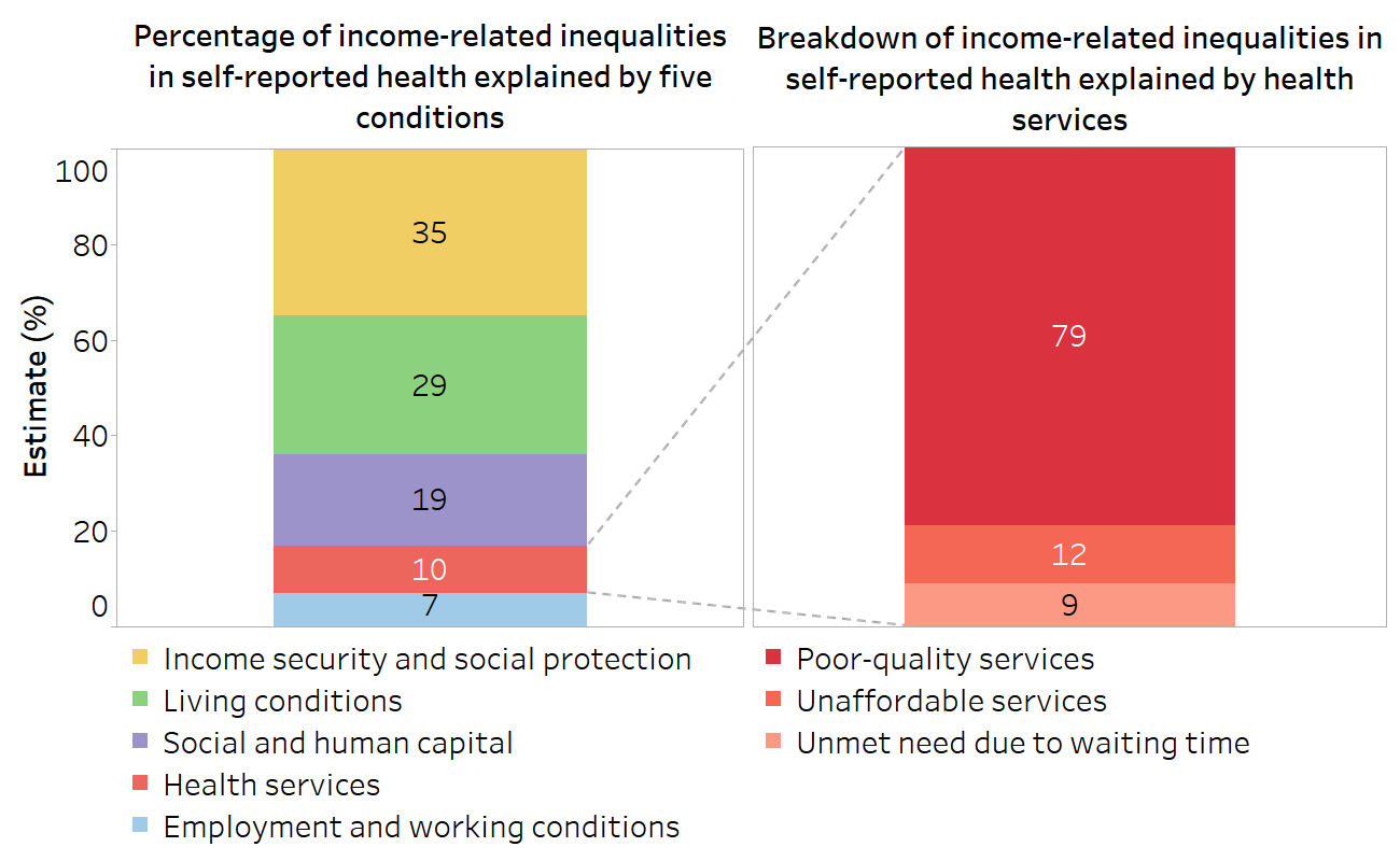
Source: derived from WHO Regional Office for Europe European health equity status report (15), with data sourced from the European Quality of Life Surveys for 2003–2016 (16).
Decomposition methods offer valuable insights, but there are challenges, including selection bias, differential measurement bias and confounding, which prevent causal interpretation derived from O–B decomposition. To overcome some of these limitations, a novel decomposition method has been proposed that involves the comparison of observed and counterfactual scenarios using a variation of the O–B method (17).
Measures of inequality using individual-level data
Research questions that seek to understand the extent of dispersion of health indicators across all individuals in a population or the level of health inequality based on individual characteristics require the analysis of individual-level data (rather than disaggregated data, or data broken down by population subgroups). This section explores the Gini coefficient to assess dispersion (which considers the distribution of a health indicator across individuals, irrespective of social characteristics) and measures of health inequality at the individual level (the association between health and socioeconomic status).
Gini coefficient
One approach to measuring dispersion of a health indicator across all individuals in a given population or setting is to use the Gini coefficient. This measure is used extensively in the field of economics to measure income inequality, but a Gini-like measure can also be used to measure the distribution of a health indicator (18).
When applied to health, Gini is a measure of dispersion that does not take into account the social position of individuals.
The measure is derived from the Lorenz curve, which plots the cumulative proportion of the health indicator against the cumulative proportion of the population, ranked from the sickest on the left to the healthiest on the right (Figure 25.4) (1). If all individuals have the same health (i.e. the cumulative proportion of the population is exactly matched to the cumulative proportion of health), the Lorenz curve runs along the 45-degree line. If there is variation in how health is distributed across individuals in the population, the Lorenz curve lies below the 45-degree line. The greater the variation of health in the population, the further the Lorenz curve lies below the 45-degree line.
FIGURE 25.4. Lorenz curve of health
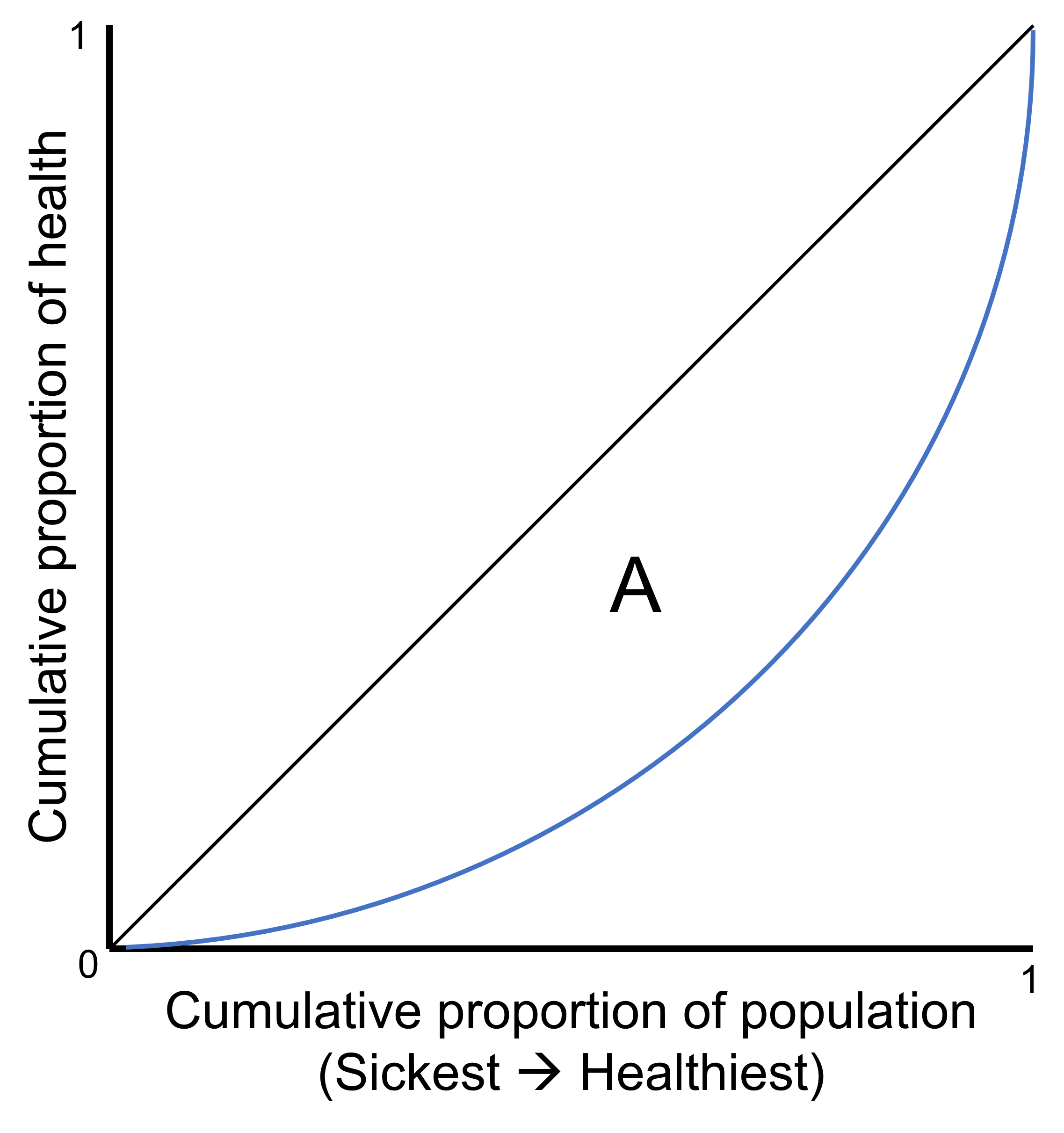
The black 45-degree line represents a situation of equality. The blue line represents the Lorenz curve, a situation of inequality. Gini coefficient is calculated as twice the area (A) between the 45-degree line and the Lorenz curve.
The Gini coefficient is twice the area (A) between the 45-degree line and the Lorenz curve. The Gini coefficient takes values between 0 and 1, with 0 being no dispersion and 1 being complete dispersion (i.e. all sickness is concentrated in one individual). This can be shown as a percentage ranging between 0% and 100%, referred to as the Gini index. See Annex 16 for an example of using Gini to measure dispersion in stunting among children in Kenya.
The Gini coefficient value becomes more meaningful if it is used to compare across time points, indicators and/or groupings of individuals or settings, to give an understanding of how the extent of dispersion has changed over time or varies across indicators and areas.
Slope index of inequality and concentration index
The slope index of inequality (SII), RII, absolute concentration index (ACI) and relative concentration index (RCI) (see Chapter 21) are summary measures of health inequality in relation to socioeconomic status (e.g. wealth or educational attainment). In addition to measuring the level of health inequality across population subgroups, they can also be used to measure inequality across individuals in a population.
Individuals are ranked from the most disadvantaged (rank 0) to the most advantaged (rank 1). This ranking can be based on a continuous measure, such as the wealth index calculated within Demographic and Health Surveys (DHS), or on a categorical measure, such as wealth quintiles or education level. The relative rank of individuals is calculated, with individuals ordered based on the socioeconomic variable and accounting for the individual sample weight in the case of data from a survey (if the data are not collected via a survey, individuals are assigned the same weight). The calculation method for SII, RII, ACI and RCI then proceeds as described in Chapter 21. Ultimately, the calculation yields a value that describes the level of inequality across all individuals from the most-advantaged to the most-disadvantaged. See Annex 17 for an example of measuring health inequality based on individual socioeconomic status.
The use of individual-level data also enables the measurement of health inequality while controlling for multiple factors, by including these factors as independent variables in the regression model used to calculate SII, RII, ACI and/or RCI. For example, Table 25.4 shows the results of a study of education-related inequalities in self-reported COVID-19 vaccination across 90 countries using SII adjusted for other individual characteristics. The gap in vaccination prevalence between the most and least educated individuals was 16.4 percentage points if no other factors were taken into account (unadjusted model) and 11.9 percentage points when characteristics including age, COVID-19-like symptoms, gender, health risk factors, household overcrowding and place of residence were controlled for (adjusted model) (19).
TABLE 25.4. Unadjusted and adjusted slope index of inequality: self-reported receipt of COVID-19 vaccine, by education level, globally and by country income group
| Number of countries | Median slope index of inequality, percentage points (95% CI) | ||
|---|---|---|---|
| Unadjusted | Adjusted | ||
| Global | 90 | 16.4 (13.4–19.3) | 11.9 (10.2–13.4) |
| High-income countries | 33 | 10.3 (7.3–12.2) | 6.9 (6.0–8.3) |
| Upper-middle-income countries | 29 | 21.4 (17.3–24.5) | 14.5 (12.9–17.1) |
| Low-income and lower-middle-income countries | 28 | 19.5 (14.2–26.6) | 13.3 (11.1–18.1) |
CI, confidence interval.
Source: derived from Bergen et al. (19), with data sourced from the 1 June to 31 December 2021 period of the University of Maryland Social Data Science Center Global COVID-19 Trends and Impact Survey.
Extensions to the concentration index
The extended concentration index allows attitudes to inequality to be made explicit (i.e. taking into account that societies are not equally averse or tolerant to inequality) and to see how the level of inequality changes as the attitude to inequality changes (1, 20). This is identical to the standard concentration index (ACI and RCI), except for the addition of a weighting function, which allows the user to determine how much weight to give to the poorest or richest individuals. A weighting of 2 is equal to the standard concentration index; a weighting of more than 2 increases weight attached to the poorest individuals. For example, the weight attached to the health of a very poor individual can be increased, and consequently the weight attached to the health of richer individuals will decrease. In a setting where the health of poor people is much worse than that of the rest of the population, such weighting will increase the magnitude of the measured inequality and therefore bring more attention to where improvements in health should be disproportionately concentrated among the poorest people.
The achievement index is another application of the concentration index, in which both health inequality and the overall mean are captured (1, 20). The achievement index is defined as a weighted average of the health levels of all people in the sample, in which higher weights are attached to poorer people than to wealthier people. Consider the example of comparing wealth-related inequality in mortality rates among children aged under five years across two countries, where both countries have the same overall level of under-five mortality but one has an unequal distribution across income groups to the disadvantage of poor people, and the other country has an equal distribution. Even though the mean is the same in the two countries, the achievement index will reflect the level of inequality and be lower than the mean in the country with pro-rich inequality.
Both the extended concentration index and the achievement index can be computed using both disaggregated data and individual-level data.
Geospatial analysis
Geospatial data and geospatial analysis can be used to answer research questions about how environmental and spatial factors influence health inequalities. Geospatial data are data about objects, events or other features that have a location on the surface of the earth (see Chapter 16). Geospatial analysis uses these spatial data and statistical techniques to uncover patterns, relationships and trends within geographic areas. Geospatial analysis is particularly relevant for the study of health inequalities because space is a determinant of exposure to environmental, zoonotic or human risk factors; poverty, educational achievement and other social determinants of health tend to be distributed unevenly in space; and health-care resources tend to be clustered in urban centres. This section discusses several applications of geospatial analysis for inequality monitoring: model-based geostatistics, distance or proximity analysis, and cluster analysis. There are also many other types of geospatial analysis techniques that can be applied to monitoring health inequalities (21).
Model-based geostatistics
The term “spatial statistics” is used to describe a wide range of statistical models and methods for the analysis of spatially referenced data. Within spatial statistics, model-based geostatistics refers to the application of general statistical principles of modelling and inference (22). Model-based geostatistics can be used to predict or forecast health indicator estimates and identify areas or populations of increased risk or need. For example, a geostatistical model could be used to predict and map malaria prevalence based on environmental factors such as altitude, rainfall, temperature and demographic factors such as place of residence and economic status of households.
Geostatistical models use three types of data: indicator data (e.g. number of people who test positive for a disease), location data (the set of locations at which the indicator data are obtained), and covariate data (variables deemed to be associated with the indicator of interest, with their aim in the model to assist the prediction of the indicator at unsampled locations). The basic premise behind this modelling is that if there is a connection between where people live and a health intervention or outcome, then that health intervention or outcome could be estimated in areas based on geospatial data about the environment and demographics. Box 25.3 describes an example from the DHS Program, where health indicators are estimated at 5 × 5 km resolutions. The accuracy of the estimates produced depends on the quality, sample sizes and granularity of the original health indicator data and the ability to link them to high-resolution geospatial data strongly associated with the original health indicator data.
BOX 25.3. DHS Program spatial data repository
DHS are designed to provide reliable estimates of survey indicators primarily at the national level. To better address the need for fine spatial and lower-level (district) estimates, geospatial modelling has become increasingly popular. The DHS Program has made publicly available a standard set of spatially modelled surfaces via the DHS Program Spatial Data Repository, which estimates various development indicators at 5 × 5 km resolutions. These maps are produced using geostatistical methods with publicly available georeferenced data from DHS and other spatial data sources (23). A series of DHS spatial analysis reports supplement other DHS reports to provide health statistics estimates at more granular levels.
For example, Figure 25.5 shows geospatially modelled immunization coverage in children in Ethiopia, based on the 2019 DHS, indicating higher immunization coverage in the western areas of the country. Such maps can be used to monitor and evaluate immunization programmes and inform decision-making about future interventions in low-coverage areas.
FIGURE 25.5. Geospatial modelling and uncertainty: immunization coverage with a third dose of diphtheria, tetanus toxoid and pertussis vaccine at the 5 × 5 km area, Ethiopia
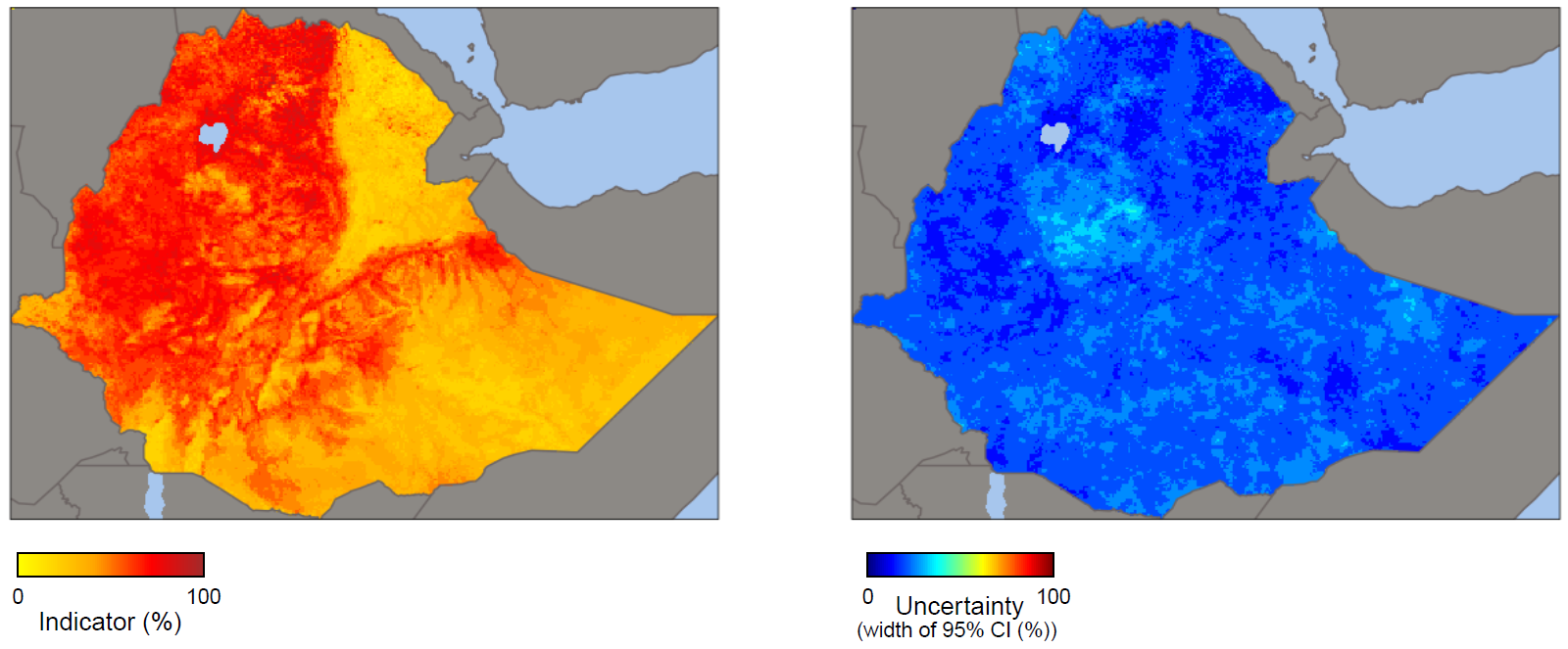
These maps were not produced by WHO. The designations employed and the representation of countries and areas in these maps may be at variance with those used by WHO and do not imply the expression of any opinion whatsoever on the part of WHO concerning the legal status of any country, territory, city or area or of its authorities, or concerning the delimitation of its frontiers or boundaries.
Uncertainty was measured using the width of the 95% confidence intervals (CIs).
Source: derived from the DHS Program Spatial Data Repository (23), with data sourced from the 2019 Demographic and Health Surveys.
Distance/proximity and cluster analyses
Distance and proximity analyses involve measuring the spatial relationships between geographic features or locations. They quantify the physical separation of locations (e.g. health-care facilities, population centres or environmental hazards), which supports the equitable planning of health facilities and access to health care. Distance analysis focuses on quantifying the physical separation between these locations. Proximity analysis examines the relative closeness or accessibility of one location to another. Often travel distance or travel time are used for these analyses rather than physical (Euclidean) distance. When analysing health inequalities, these methods can be used to assess, for example, the accessibility and availability of health-care services across different geographic areas, helping to highlight populations that are disadvantaged and areas where interventions are needed to improve equity in health-care delivery. Additionally, distance and/or proximity analysis can be used to study the relationship between environmental factors (e.g. pollution sources or water bodies) and health outcomes, helping to identify spatial factors associated with health inequalities.
Spatial autocorrelation is a measure of the similarity of nearby observations. Positive spatial autocorrelation occurs when observations with similar values are closer together (i.e. clustered). Negative spatial autocorrelation occurs when observations with dissimilar values are closer together (i.e. disbursed). Cluster analysis uses tests of spatial autocorrelation to identify groups, or clusters, based on the similarity of certain characteristics. It looks at the spatial distribution of health indicators to identify hotspots (i.e. areas of high concentration of the health indicator, such as areas with high cardiovascular disease) and coldspots (i.e. areas of low concentration of the health indicator, such as areas that have poor accessibility to health care) – both of which are useful for targeting interventions. The goal of cluster analysis is to partition data points into distinct groups where observations within each group are more similar to each other than to those in other groups. In the context of geospatial data analysis, cluster analysis can be applied to identify geographic areas or communities that exhibit similar patterns of health outcomes or risk factors. Analysing geospatial data related to disease prevalence rates, socioeconomic indicators or environmental exposures can be used to group communities, neighbourhoods or subnational regions with similar health profiles, revealing spatial patterns of inequalities and highlighting areas where certain population groups may be disproportionately affected by poor health outcomes or lack of health care interventions. For example, the average shortest distance travelled from settlements to medical facilities has been analysed to calculate spatial accessibility in 2859 counties in China (24).
Small-area estimation
To understand how a health indicator may vary across small geographic areas or demographic and socioeconomic groups (for which data may be sparse or unavailable), small-area estimation can be used to generate reliable estimates. This methodological approach can be used in health inequality monitoring to produce estimates at a resolution that enables policy-makers to identify areas or populations at greatest risk.
As mentioned in previous chapters, inequality monitoring requires data disaggregated by demographic, socioeconomic and geographic characteristics. Household survey data (a primary data source to assess inequalities in health-care access and health burden in low-income settings) are usually designed to produce reliable estimates at the national level or by broad regions. In most subnational areas, therefore, sample sizes to produce direct survey estimates of health-care access or disease burden disaggregated by sociodemographic groups or small geographic areas are often small or there are no data. Rather than substantially increasing sample size in household surveys, which would be extremely costly and logistically challenging, small-area estimation offers the possibility to incorporate pre-existing data. By “borrowing strength” from auxiliary information included in large datasets such as census data or routinely collected programmatic data, small-area estimation can enhance the precision of estimates for small areas or specific groups, without any additional data collection effort (25–28). Geospatial modelling (see above) can also be used in small-area estimation to improve predicted estimates, particularly when high-quality census or administrative data are not available. An example of the application of small-area estimation is given in Box 25.4.
BOX 25.4. Small-area estimation of measles immunization coverage in Nigeria
Small-area estimation has been used in the analysis of measles-containing vaccine (MCV1) coverage among children aged 12–23 months in Nigeria (29), using data from the 2018 DHS. Traditional direct estimates revealed significant variance in vaccination rates between states (i.e. first administrative subdivisions) and across different districts (local government areas) within states (i.e. second administrative subdivisions). Some districts, however, were lacking sufficient sample size for the reliable estimation of vaccination rates. Figure 25.6 shows the cluster-level MCV1 coverage data from the survey at the state level. Many clusters were sampled in the southern, south-western, northern and north-western states, but data are sparse in the north-east. As a result, direct estimates of MCV1 coverage would likely be unstable at the state level and would be missing at lower (e.g. district) levels.
FIGURE 25.6. Cluster-level map of measles-containing vaccine (MCV1) coverage, Nigeria
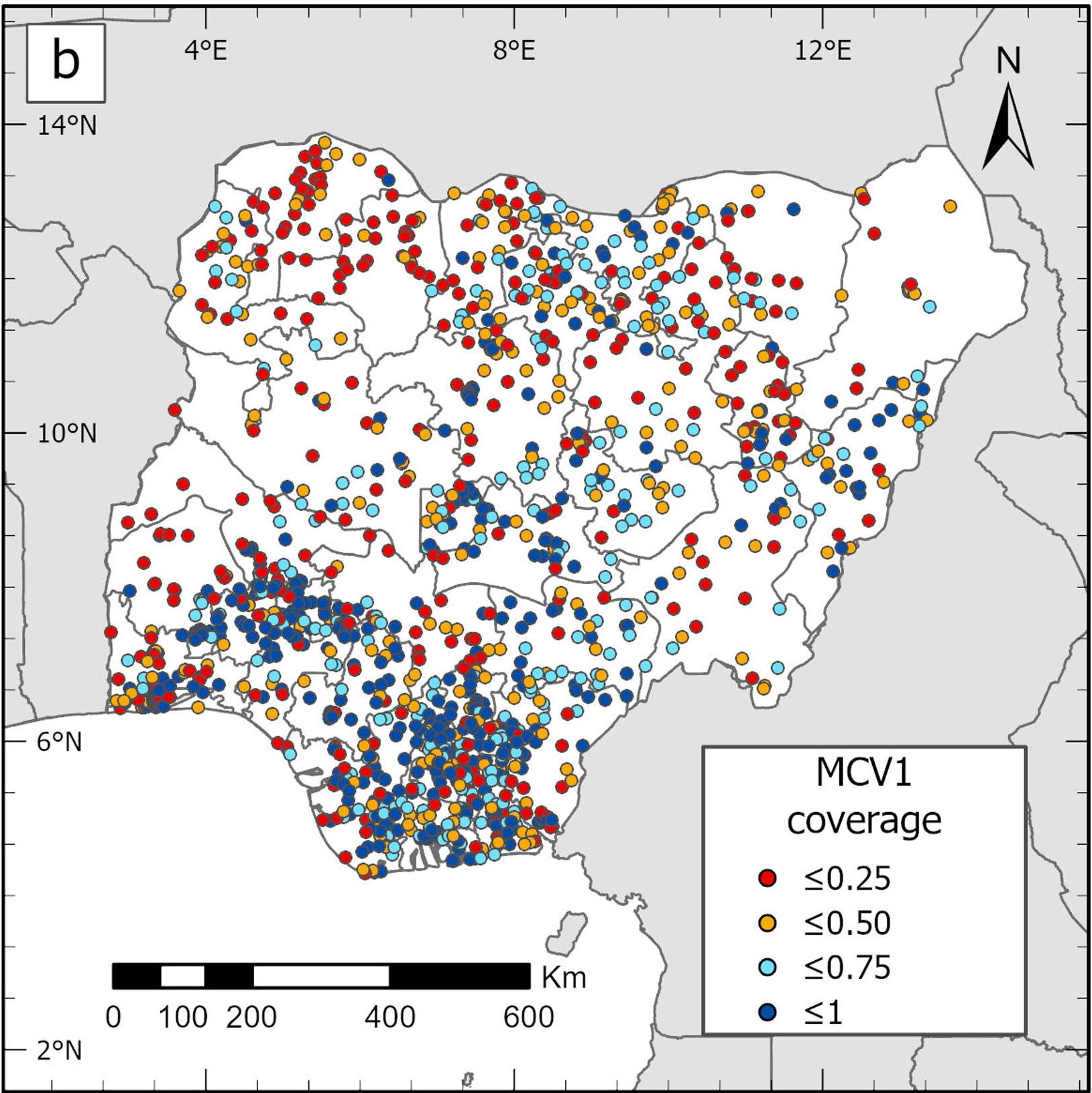
This map was not produced by WHO. The designations employed and the representation of countries and areas in this map may be at variance with those used by WHO and do not imply the expression of any opinion whatsoever on the part of WHO concerning the legal status of any country, territory, city or area or of its authorities, or concerning the delimitation of its frontiers or boundaries. MCV1 coverage is measured as a percentage.
Source: derived from Utazi et al. (29), with data sourced from the 2018 Demographic and Health Surveys.
Using small-area estimation, researchers integrated a suite of geospatial socioeconomic, environmental and physical covariates (including population size, travel time to nearest health facility, poverty rates, nightlight intensity and land surface temperature) and laboratory-supported measles surveillance data, and also used spatial autocorrelation to model and predict vaccination coverage at the 1 × 1 km resolution at the district and the state level (Figure 25.7), ultimately identifying specific districts with critically low vaccination rates. This targeted approach can facilitate the design of focused immunization campaigns.
FIGURE 25.7. Modelled estimates of measles-containing vaccine (MCV1) coverage, Nigeria
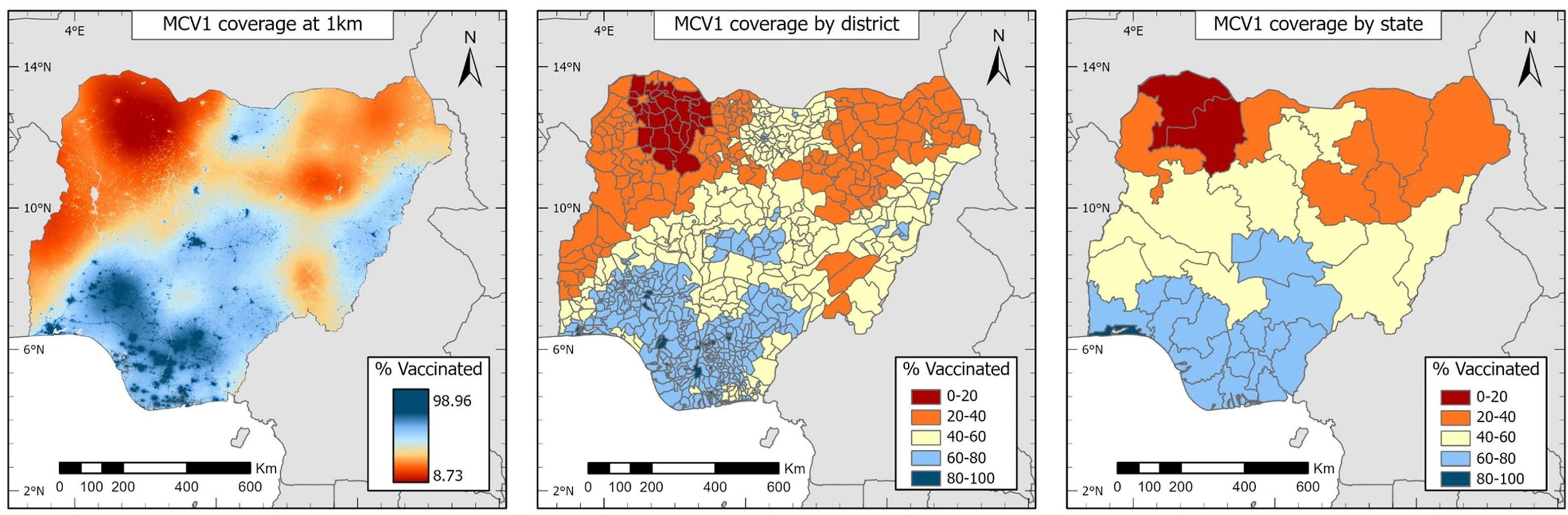
These maps were not produced by WHO. The designations employed and the representation of countries and areas in these maps may be at variance with those used by WHO and do not imply the expression of any opinion whatsoever on the part of WHO concerning the legal status of any country, territory, city or area or of its authorities, or concerning the delimitation of its frontiers or boundaries.
Source: derived from Utazi et al. (29), with data sourced from the 2018 Demographic and Health Surveys.
Ecological analysis
Investigating how health determinants or factors at a population level can affect health outcomes can be achieved through ecological analysis. Ecological analyses are based on aggregated or grouped data, such as examining relationships between a health indicator and a health determinants or exposure at a population level. In ecological studies, data are analysed at an aggregate level, such as neighbourhoods, cities, subnational regions or countries. These studies can provide insights into how various environmental, social or policy factors may influence health indicators within a population group (see Box 25.5 for examples of health determinant indicators). Ecological studies would be useful to explore, for example, the relationship between air pollution levels and respiratory disease rates; how economic status is related to obesity prevalence; or the impact of smoke-free legislation on smoking rates.
In inequality monitoring, ecological studies can be used to highlight the importance of addressing certain determinants to improve the health indicator of interest. They can also assess large-scale impacts of an intervention or a policy on population health. For example, ecological analyses of the relationship between economic status and immunization rates could be performed using data collected before and after the introduction of a national vaccination campaign, to see whether the campaign was successful in reducing or eliminating economic-related inequality in immunization coverage. Ecological studies are valuable because they can be done relatively easily and quickly using indicator estimates at the subnational or national level.
BOX 25.5. Examples of determinants of health for ecological analysis
The following are examples of health determinant indicators for conducting ecological analysis at a national level. The choice of determinant depends on the research question and data availability. This list is for illustrative purposes only and is not exhaustive.
Physical environment:
air pollution;
population with access to electricity;
households that live in overcrowded dwellings;
population using basic sanitation.
Livelihood and skills:
population living below the poverty line;
population living in multidimensional poverty;
urban population living in slums;
primary school completion rate;
unemployment rate.
Health system coverage and inputs:
government health expenditure per capita;
universal health coverage service coverage index;
health worker density;
health facility density;
out-of-pocket health expenditure.
Social and economic inclusion:
gender inequality index;
Gini index for income inequality;
population experiencing discrimination.
Statistical analysis is used to explore relationships between the health indicator and health determinant. Common techniques include correlation analysis (measuring the strength of the linear or nonlinear (monotonic) relationship between the two variables and computing their association) and regression analysis (see above). An example of the use of regression models to analyse associations between gender inequality and childhood immunization is shown in Box 25.6.
BOX 25.6. Associations between gender inequality and childhood immunization at the subnational level
Gender inequality is increasingly recognized as a key determinant of childhood immunization coverage and health equity. In an ecological study, logistic regression models were used to estimate the association between two immunization indicators (prevalence of unvaccinated, or zero-dose, children and DTP3 immunization coverage) and gender inequality, at the subnational level across 57 countries (30).
Human development has been measured using the human development index (HDI), which summarizes the level of development across education, health and standard of living (31). Gender inequality was measured using the subnational gender development index, which is the ratio of HDI among men to HDI among women within a subnational region.
Two regression models were used to analyse the association between gender inequality and childhood immunization – the first was a simple regression model that had no further variables (i.e. unadjusted), and the second included other factors associated with immunization coverage such as urban population and human development indicators (i.e. adjusted).
The results showed that in subnational regions with higher gender inequality, zero-dose prevalence odds were 1.7 times higher compared with subnational regions with lower inequality controlling for other factors included in the model; the odds of DTP3 immunization coverage were 39% lower (Table 25.5). This demonstrates that within-country variation in gender inequality is associated with immunization coverage at the subnational level and suggests that gender inequality may be one of many drivers of subnational inequalities in coverage.
TABLE 25.5. Odds ratios: zero-dose prevalence and immunization coverage with a third dose of diphtheria, tetanus toxoid and pertussis vaccine (DTP3), by subnational gender development index category in 702 subnational regions across 57 countries
| Odds ratio (95% CI) | ||
|---|---|---|
| Unadjusted | Adjusted | |
| Zero-dose children | 2.637 (2.122–3.275) | 1.742 (1.384–2.193) |
| DTP3 immunization coverage | 0.437 (0.364–0.524) | 0.614 (0.505–0.746) |
CI, confidence interval.
Source: derived from Johns et al. (30), with data sourced from 2010–2019 subnational regional estimates published by the Global Data Lab.
The major limitation of ecological analyses is that because data are not being analysed at the individual level, care is needed in interpretation to avoid ecological fallacy (see Chapter 18). Although ecological analysis can identify associations, they cannot establish causality at the individual level. It is important to be aware of potential confounding factors that may influence the observed relationships.
Measuring between-country inequality
Answering research questions related to quantifying the overall level of inequality in a health indicator between countries can be achieved by measuring between-country inequality. Measuring between-country inequality, unlike within-country inequality, does not quantify inequalities based on demographic or socioeconomic characteristics (i.e. dimensions of inequality); rather, it simply seeks to quantify the variation across countries. It uses national average data rather than disaggregated data.
Many of the summary measures of inequality described in Chapters 19–21 used for measuring within-country inequalities can also be used to quantify inequalities between countries. The calculation methods described in these chapters can be used, replacing subgroup estimates for country estimates, and subgroup population sizes for country population sizes. For example, inequality in a health indicator across a group of countries can be assessed as the difference or the ratio between the countries with the highest and lowest health indicator estimates. To take all countries (and their population sizes) into account, between-group variance, between-group standard deviation, coefficient of variation and weighted mean difference from mean could be used to quantify the level of variance between all countries and the overall mean. An example of the calculation of the weighted mean difference from a best-performing subgroup (MDBW; also known as international shortfall inequality when applied to measuring between-country inequality) is highlighted in Box 25.7. The Gini coefficient (see earlier) can also be used to measure dispersion in a health indicator across countries.
BOX 25.7. Example calculation of international shortfall inequality
When measuring between-country inequality, MDBW (international shortfall inequality) is defined as the weighted average of the deviation of each country’s indicator estimate from the highest estimate, weighted by country population. It measures the absolute difference, or the degree of shortfall, from the highest attained estimate. It can be turned into a relative measure by dividing the result by the highest estimate.
In the context of measuring between-country inequality, MDBW is calculated as
\[\sum P_{country} \left| y_{best} - y_{country} \right|\]
where \(y_{country}\) is the country indicator estimate, \(y_{best}\) is the highest estimate (e.g. the best-performing country or the top fifth percentile of countries), and \(P_{country}\) is the country’s population share out of the total population of all countries.
Table 25.6 shows an example of the calculation of MDBW for a set of 19 middle-income European countries. It shows that, on average, these countries had a life expectancy of 4.6 years less than Albania (the country among them with the highest life expectancy).
TABLE 25.6. Steps to calculate mean difference from best-performing subgroup (weighted): life expectancy at birth in 19 middle-income countries in the WHO European Region
| Country |
Life expectancy at birth (years) [A] |
Population size (thousands) [C] |
Population share [E = C / D] |
Difference between highest estimate and country estimate [F = B – A] |
Weighted difference (years) [G = E × F] |
|---|---|---|---|---|---|
| Albaniaa |
76.4 [B] |
2856 | 0.007 | 0.0 | 0.000 |
| Armenia | 73.0 | 2791 | 0.007 | 3.4 | 0.024 |
| Azerbaijan | 72.9 | 10 313 | 0.026 | 3.5 | 0.091 |
| Belarus | 73.1 | 9578 | 0.024 | 3.3 | 0.079 |
| Bosnia and Herzegovina | 74.8 | 3271 | 0.008 | 1.6 | 0.013 |
| Bulgaria | 71.3 | 6886 | 0.017 | 5.1 | 0.087 |
| Georgia | 71.2 | 3758 | 0.009 | 5.2 | 0.047 |
| Kazakhstan | 70.3 | 19 196 | 0.048 | 6.1 | 0.293 |
| Kyrgyzstan | 72.2 | 6528 | 0.016 | 4.2 | 0.067 |
| Montenegro | 74.7 | 628 | 0.002 | 1.7 | 0.003 |
| North Macedonia | 73.0 | 2103 | 0.005 | 3.4 | 0.017 |
| Republic of Moldova | 69.6 | 3062 | 0.008 | 6.8 | 0.054 |
| Russian Federation | 70.0 | 145 103 | 0.361 | 6.4 | 2.310 |
| Serbia | 72.8 | 7297 | 0.018 | 3.6 | 0.065 |
| Tajikistan | 71.8 | 9750 | 0.024 | 4.6 | 0.110 |
| Türkiye | 75.3 | 84 775 | 0.211 | 1.1 | 0.232 |
| Turkmenistan | 69.1 | 6342 | 0.016 | 7.3 | 0.117 |
| Ukraine | 70.9 | 43 531 | 0.108 | 5.5 | 0.594 |
| Uzbekistan | 72.2 | 34 081 | 0.085 | 4.2 | 0.357 |
| Total |
401 849 [D] |
Mean difference from best-performing subgroup (weighted) = 4.6 |
a Highest estimate (Albania).
Source: data from 2021 WHO Global Health Estimates (32).
A higher MDBW value indicates greater between-country inequality, or a higher absolute difference between the best-performing country and the other countries. MDBW is measured in the same unit as the health indicator. Like other summary measures, MDBW is more meaningful when used to compare inequality across different time points, different populations within countries (e.g. females and males), and different groupings of countries (e.g. regions or World Bank income groupings).
References
1. O’Donnell O, Van Doorslaer E, Wagstaff A, Lindelow M. Analyzing health equity using household survey data: a guide to techniques and their implementation. Washington, DC: World Bank; 2008 (https://openknowledge.worldbank.org/entities/publication/8c581d2b-ea86-56f4-8e9d-fbde5419bc2a, accessed 9 August June 2024).
2. Sunil Rao J. Statistical methods in health disparity research. Boca Raton, FL: CRC Press; 2023.
3. Szklo M, Nieto FJ. Epidemiology: beyond the basics. Burlington, MA: Jones & Bartlett Learning; 2019.
4. Bauer GR, Churchill SM, Mahendran M, Walwyn C, Lizotte D, Villa-Rueda AA. Intersectionality in quantitative research: a systematic review of its emergence and applications of theory and methods. SSM Popul Health. 2021;14:100798. doi:10.1016/j.ssmph.2021.100798.
5. Piccininni M, Konigorski S, Rohmann JL, Kurth T. Directed acyclic graphs and causal thinking in clinical risk prediction modeling. BMC Med Res Methodol. 2020;20(1):1–9. doi:10.1186/s12874-020-01058-z.
6. Peduzzi P, Concato J, Kemper E, Holford TR, Feinstein AR. A simulation study of the number of events per variable in logistic regression analysis. J Clin Epidemiol. 1996;49(12):1373-1379. doi:10.1016/s0895-4356(96)00236-3.
7. Schisterman EF, Perkins NJ, Mumford SL, Ahrens KA, Mitchell EM. Collinearity and causal diagrams: a lesson on the importance of model specification. Epidemiology. 2017;28(1):47. doi:10.1097/EDE.0000000000000554.
8. Greenland S, Daniel R, Pearce N. Outcome modelling strategies in epidemiology: traditional methods and basic alternatives. Int J Epidemiol. 2016;45(2):565. doi:10.1093/ije/dyw040.
9. Explorations of inequality: childhood immunization. Geneva: World Health Organization; 2018 (https://iris.who.int/handle/10665/272864, accessed 12 June 2024).
10. Hosseinpoor AR, Parker LA, Tursan d’Espaignet E, Chatterji S. Socioeconomic inequality in smoking in low-income and middle-income countries: results from the World Health Survey. PLoS One. 2012;7(8):42843. doi:10.1371/journal.pone.0042843.
11. Rahimi E, Hashemi Nazari SS. A detailed explanation and graphical representation of the Blinder–Oaxaca decomposition method with its application in health inequalities. Emerg Themes Epidemiol. 2021;18(1). doi:10.1186/s12982-021-00100-9.
12. STEPwise approach to NCD risk factor surveillance (STEPS). Geneva: World Health Organization (https://www.who.int/teams/noncommunicable-diseases/surveillance/systems-tools/steps, accessed 19 June 2024).
13. Wagstaff A, Van Doorslaer E, Watanabe N. On decomposing the causes of health sector inequalities with an application to malnutrition inequalities in Vietnam. J Econom. 2003;112(1):207–223. doi:10.1016/S0304-4076(02)00161-6.
14. Hosseinpoor AR, Van Doorslaer E, Speybroeck N, Naghavi M, Mohammad K, Majdzadeh R, et al. Decomposing socioeconomic inequality in infant mortality in Iran. Int J Epidemiol. 2006;35(5):1211–1219. doi:10.1093/ije/dyl164.
15. Healthy, prosperous lives for all: the European Health Equity Status Report. Copenhagen: World Health Organization Regional Office for Europe; 2019 (https://iris.who.int/handle/10665/326879, accessed 12 June 2024).
16. European Quality of Life Surveys. Dublin: Eurofound (https://www.eurofound.europa.eu/en/surveys/european-quality-life-surveys-eqls).
17. Jackson JW, VanderWeele TJ. Decomposition analysis to identify intervention targets for reducing disparities. Epidemiology. 2018;29(6):825. doi:10.1097/EDE.0000000000000901.
18. Mackenbach JP, Kunst AE. Measuring the magnitude of socio-economic inequalities in health: an overview of available measures illustrated with two examples from Europe. Soc Sci Med. 1997;44(6):757–771. doi:10.1016/s0277-9536(96)00073-1.
19. Bergen N, Kirkby K, Fuertes CV, Schlotheuber A, Menning L, Mac Feely S, et al. Global state of education-related inequality in COVID-19 vaccine coverage, structural barriers, vaccine hesitancy, and vaccine refusal: findings from the Global COVID-19 Trends and Impact Survey. Lancet Glob Heal. 2023;11(2):e207–e217. doi:10.1016/S2214-109X(22)00520-4.
20. Wagstaff A. Inequality aversion, health inequalities and health achievement. J Health Econ. 2002;21(4):627–641. doi:10.1016/s0167-6296(02)00006-1.
21. Maantay JA, McLafferty S. Geospatial analysis of environmental health. Dordrecht: Springer; 2011.
22. Diggle PJ, Giorgi E. Model-based geostatistics for global public health: methods and applications. Boca Raton, FL: Taylor & Francis; 2019.
23. DHS Program. Spatial data repository. Washington, DC: United States Agency for International Development (https://spatialdata.dhsprogram.com/home/, accessed 12 June 2024).
24. Yin C, He Q, Liu Y, Chen W, Gao Y. Inequality of public health and its role in spatial accessibility to medical facilities in China. Appl Geogr. 2018;92:50–62. doi:10.1016/j.apgeog.2018.01.011.
25. Gutreuter S, Igumbor E, Wabiri N, Desai M, Durand L. Improving estimates of district HIV prevalence and burden in South Africa using small area estimation techniques. PLoS One. 2019;14(2):e0212445. doi:10.1371/journal.pone.0212445.
26. Pfeffermann D. New important developments in small area estimation. Stat Sci. 2013;28(1):40–68. doi:10.1214/12-STS395.
27. Dong TQ, Wakefield J. Modeling and presentation of vaccination coverage estimates using data from household surveys. Vaccine. 2021;39(18):2584–2594.doi:10.1016/j.vaccine.2021.03.007.
28. Wakefield J. Prevalence mapping. Wiley StatsRef: Statistics Reference Online. 2020;1–7. doi:10.1002/9781118445112.stat08238.
29. Utazi CE, Aheto JMK, Wigley A, Tejedor-Garavito N, Bonnie A, Nnanatu CC, et al. Mapping the distribution of zero-dose children to assess the performance of vaccine delivery strategies and their relationships with measles incidence in Nigeria. Vaccine. 2023;41(1):170–181. doi:10.1016/j.vaccine.2022.11.026.
30. Johns NE, Kirkby K, Goodman TS, Heidari S, Munro J, Shendale S, et al. Subnational gender inequality and childhood immunization: an ecological analysis of the subnational gender development index and DTP coverage outcomes across 57 countries. Vaccines (Basel). 2022;10(11):1951. doi:10.3390/vaccines10111951.
31. Human Development Index (HDI). New York: United Nations Development Programme (https://hdr.undp.org/data-center/human-development-index#/indicies/HDI0, accessed 31 May 2024).
32. Global Health Estimates: life expectancy and healthy life expectancy. Geneva: World Health Organization (https://www.who.int/data/gho/data/themes/mortality-and-global-health-estimates/ghe-life-expectancy-and-healthy-life-expectancy, accessed 19 August 2024).